Transient + Excitation¶

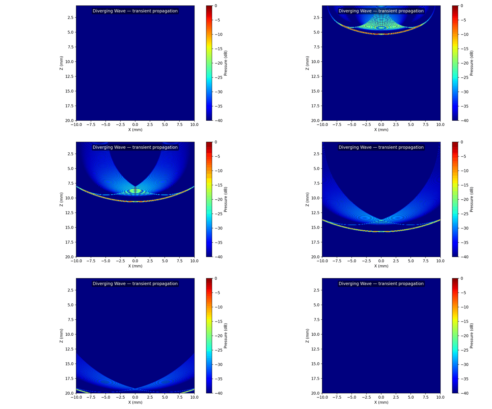
The SIR is convolved (in the frequency domain) with a user excitation pulse, giving the full time-domain pressure wavefront p(t, x, y, z). Pass one global pulse (L,) or a per-element pulse (L, E).

import numpy as np
from esdiva.emission import Emission

fs, fc, n_cycles = 200e6, tx.fc, 2
t = np.arange(0, n_cycles / fc, 1 / fs)
excitation = np.hanning(len(t)) * np.sin(2 * np.pi * fc * t)

sim = Emission(tx, fs=fs, excitation=excitation)
p, coords = sim(field_points)
# dict input : p.shape == (Nt, Nx, Ny, Nz), coords has "x","y","z","t0","dt"

p is the signed pressure in pascals (compression > 0, rarefaction < 0) for rho in kg/m³ and the excitation read as a surface velocity in m/s; it does not depend on fs. Peak negative pressure is -p.min(axis=0); take np.abs(p) or an envelope for field maps. If tx.impulse_response is set, the velocity is the full excitation ⊛ ir.

When to use¶

• Realistic pulsed propagation waveforms (DW, steered PW, focused).
• Acoustic intensity / heating maps.
• Comparing pulse shapes and their effect on the focal pattern.

See Example 4 — Diverging Wave and Example 5 — Steered Plane Wave.