Example 21: Volumetric Imaging Case Study — Matrix Probe, DW Sequence¶

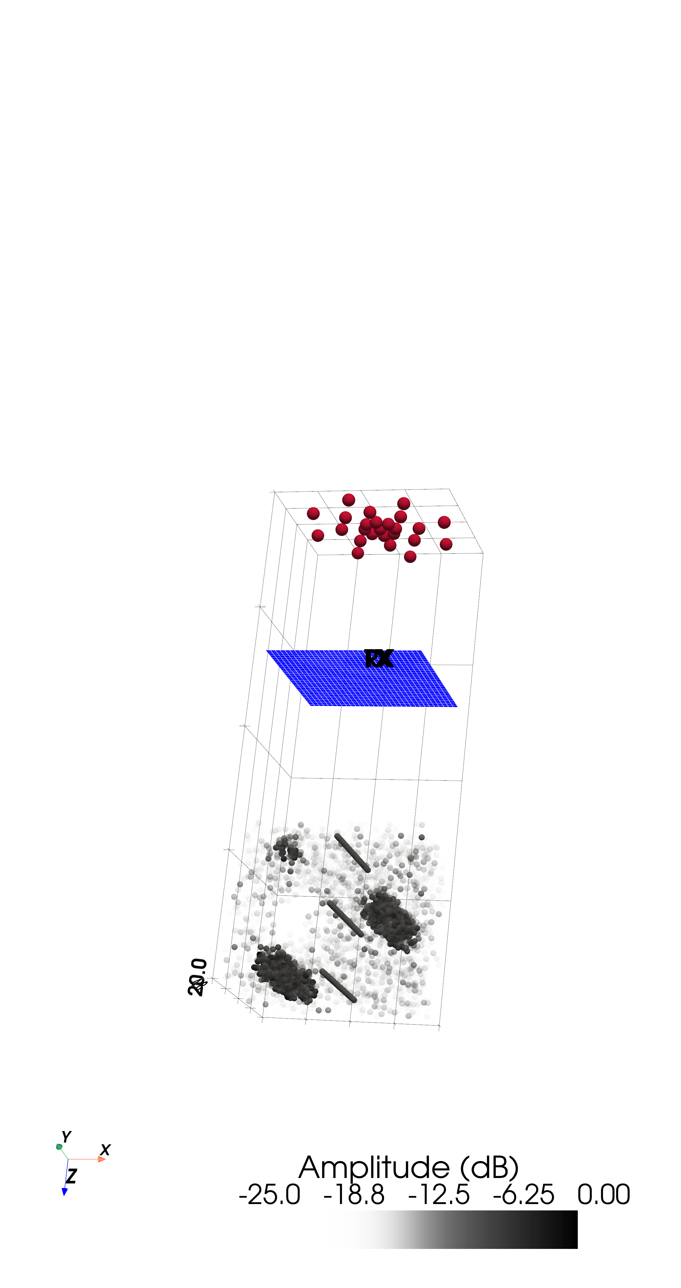
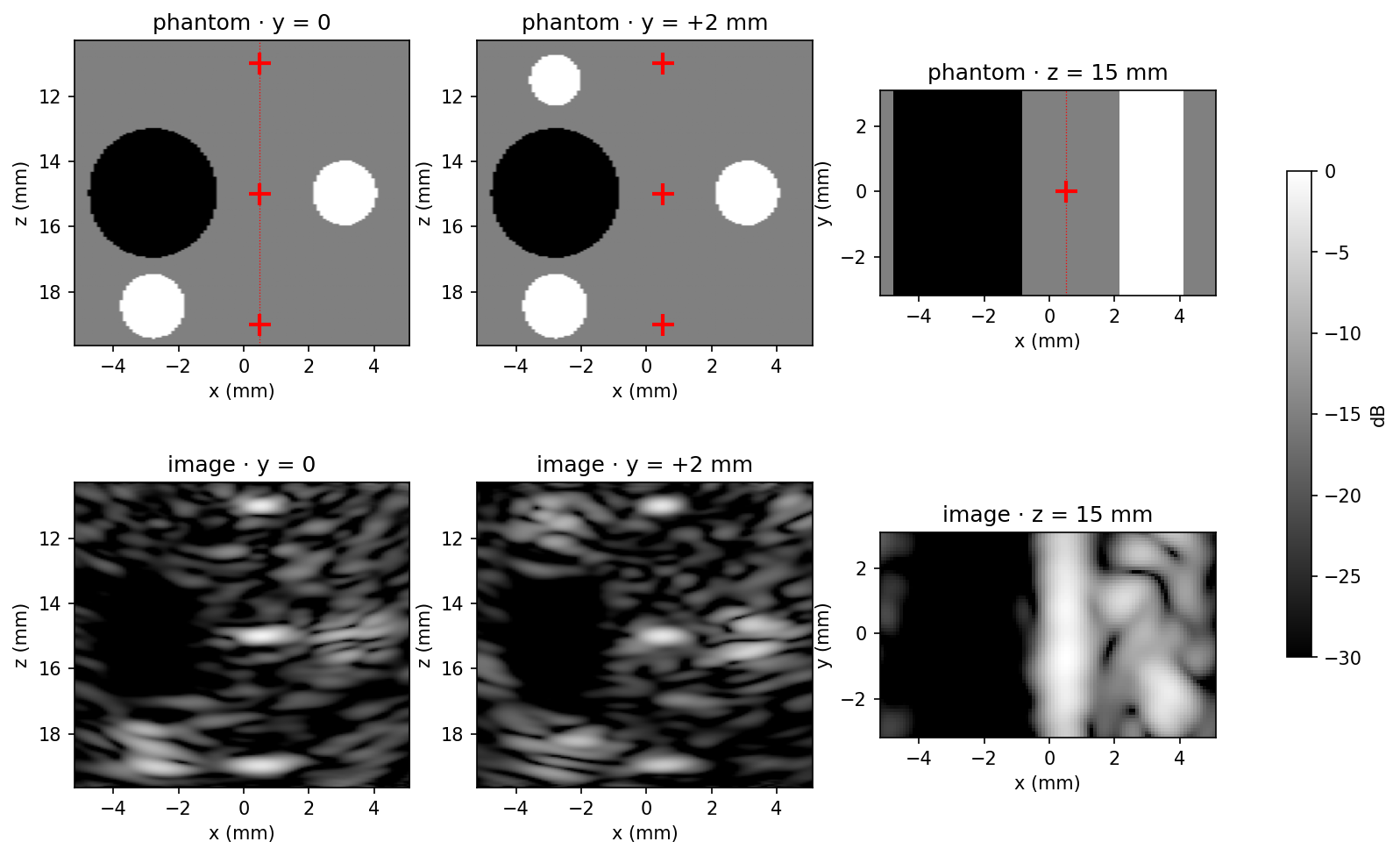
A complete, checkpointed volumetric imaging pipeline in three steps: a shared contrast-ladder phantom (anechoic cyst, ×4 lesions, elevation sphere, PSF wires + bead column), a diverging-wave transmit sequence derived per probe from the coverage rule, crash-safe RF acquisition, and per-event 3-D delay-and-sum with coherent IQ compounding. Three probe scenarios share one phantom; the default vermon (32×32, 3 MHz) runs the full pipeline in minutes.

The pipeline¶

Script	What it does
`step1_define_phantom_TX_RX.py`	All definitions in one place: scenario (probe + drive), phantom, virtual-source sequence, drive burst + piezo impulse response, beamforming grid
`step2_acquire_RF.py`	`Reception(method="spectral")`, one TX event at a time, checkpointed to `out/<scenario>/RF/` (resumable, refuses a changed config)
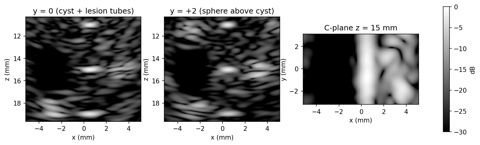
`step3_beamforming.py`	Per-event `das_volume` → Hilbert IQ → coherent compound → depth-only TGC → contrast/SNR/PSF metrics + B-mode figures

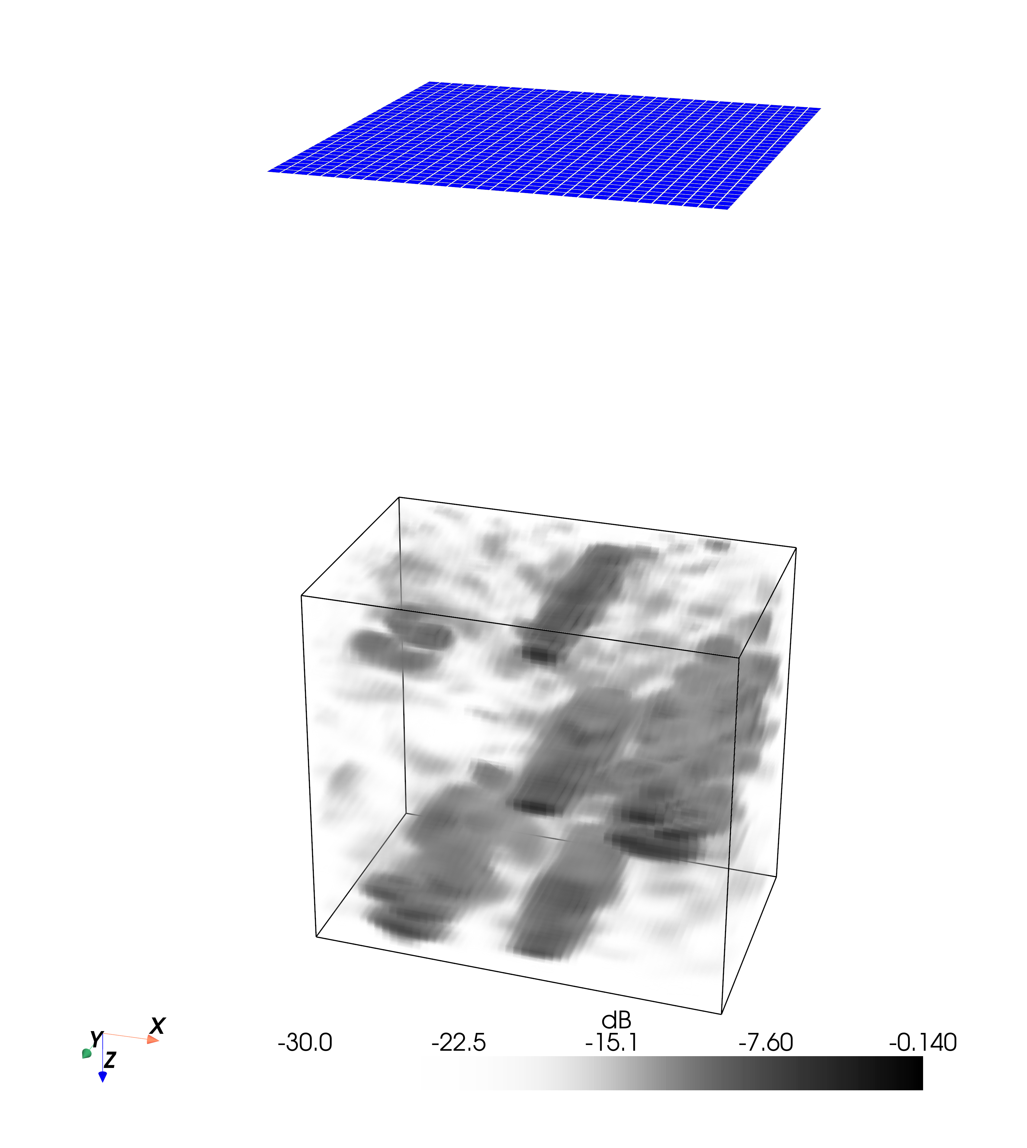
Supporting scripts: preview_phantom.py (truth + acquisition scene BEFORE the long run) and visualize_beamformed_volume.py (3-D renders from the saved IQ volume — never re-beamforms).

Output (vermon scenario)¶

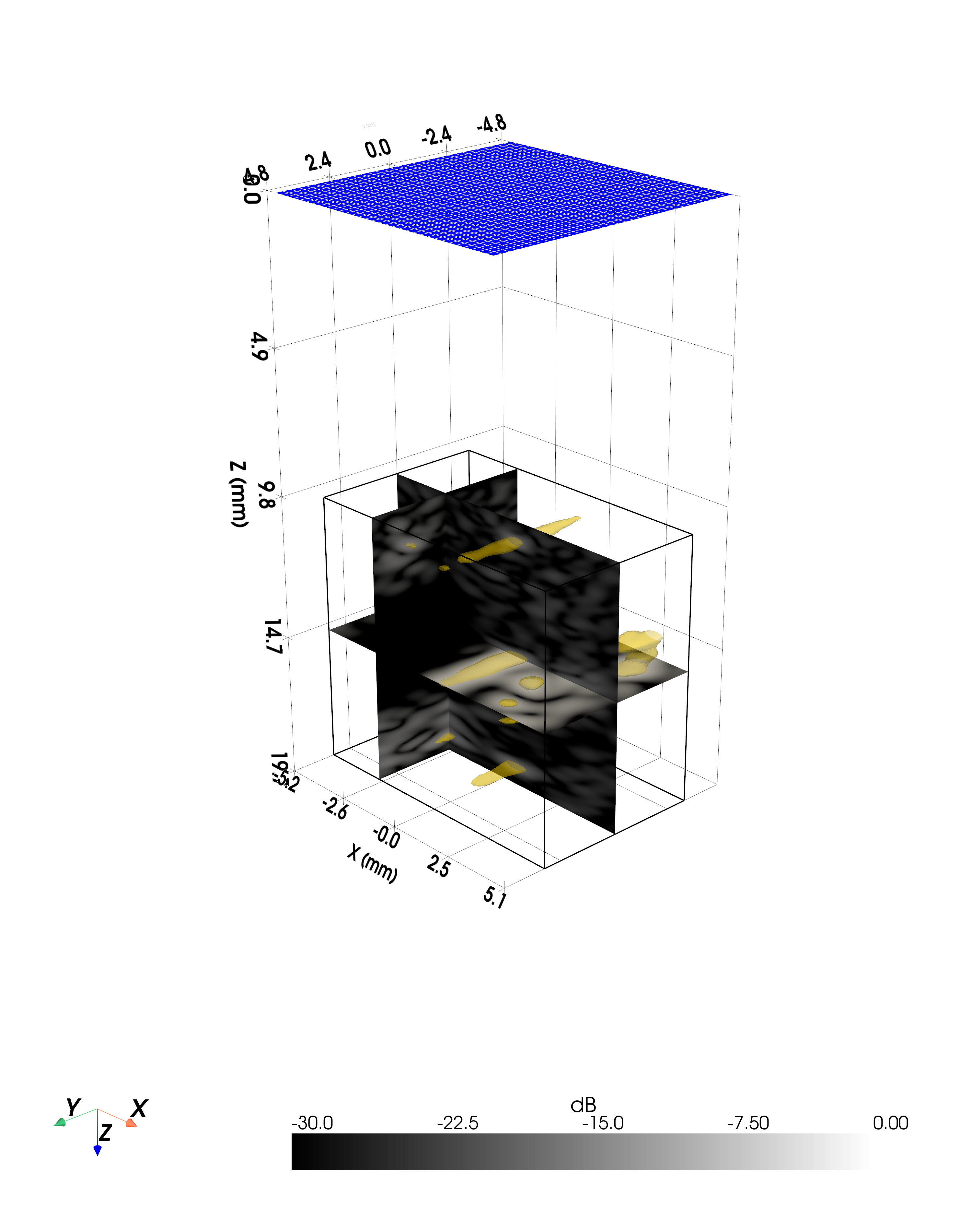
Phantom + probe + virtual sources B-mode triptych Phantom truth vs image Volume render MPR cut planes

Run it¶

uv run examples/example21_3Dphantom_volume/step2_acquire_RF.py
uv run examples/example21_3Dphantom_volume/step3_beamforming.py
# pick another probe: SCENARIO=zeus5 (or zeus10) before the commands

Where the lessons live¶

Every design rule this case study cost us — impulse responses, virtual-source coverage, phantom density, wire brightness, honest metrics — is distilled in the example folder's README.md under "Design notes & pitfalls".