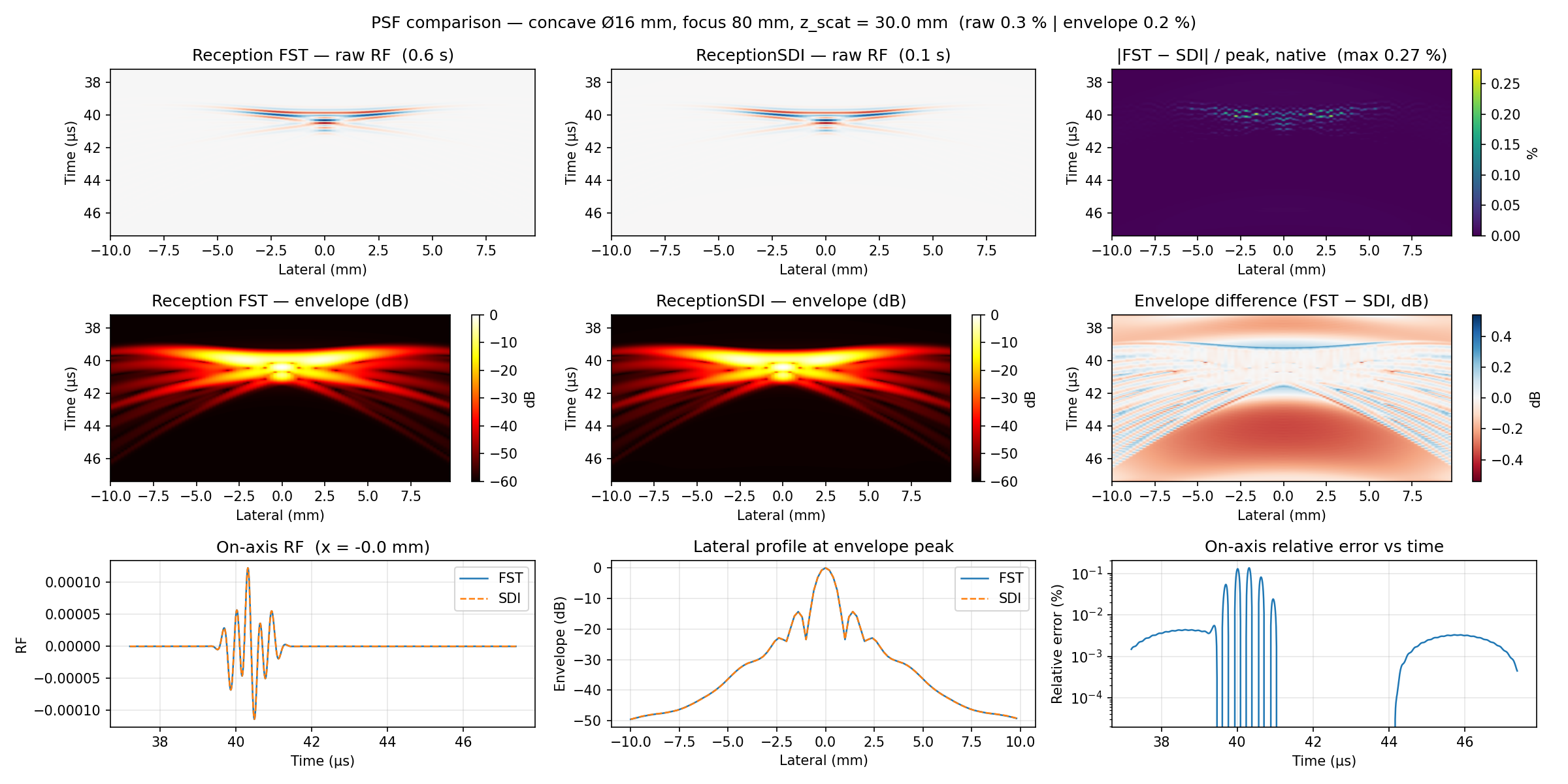
Example 6: Concave Transducer — Pulse-Echo PSF
Computes the pulse-echo point spread function (PSF) of a spherically focused
single-element transducer, comparing two methods of the one Reception class:
conventional (method="fst", Field II-style SIR convolution) and the default
PE-SDI (method="spectral"). Both agree to a fraction of a percent — the
comparison doubles as a self-validation of the reception engine.
What you will learn
- Sweeping a point scatterer laterally to build a PSF image
pulse_echo_rf(..., per_scatterer=True)— one RF trace per scatterer- Setting the transducer
impulse_response/excitationchain - Raw-RF and log-envelope comparison between backends
Output
Run it
Key code
from esdiva.reception import Reception
from esdiva.transducers import ConcaveCircularTransducer

tx = ConcaveCircularTransducer(diameter_mm=16, focus_mm=80, frequency_Hz=3e6,
                               no_sub_diameter=16)
tx.impulse_response = pulse
tx.excitation = pulse
rx = tx.copy()

sim = Reception(tx, rx, fs=100e6, c=1540)   # default method="spectral"
rf, coords = sim.pulse_echo_rf(scatterer_positions_mm, per_scatterer=True)
# rf.shape = (N_scat, E_rx, Nt) — the PSF, one trace per lateral position