Reception (RF)¶

Reception computes the pulse-echo RF scattered by point targets back onto the receive elements — the raw channel data a scanner would digitise. It is the basis for PSF, phantom, FMC, and sequence (PW/DW) imaging studies, and matches Field II to correlation ~1.0 while running >20× faster on large apertures.

One class, Reception, does everything; its method selector picks how the two-way SIR is evaluated (speed only — all give the same RF):

• "spectral" (default) — fast sparse-delta kernel via closed-form one-way SIR spectra.
• "fst" / "sdi" / "auto" — conventional Tupholme-Stepanishen sampled convolution.
• "paired" — exact but slow pedagogic reference (warns on selection).

from esdiva.reception import Reception

sim = Reception(tx, rx, fs=200e6, c=1540)             # separate TX / RX transducers
rf, coords = sim.pulse_echo_rf(scatterer_pos_mm, scatterer_amp)   # (Erx, Nt)

The physics: the pulse-echo signal is v_pe ⊛ h_tx ⊛ h_rx, with the excitation and TX/RX impulse responses carrying the band-limited pulse (same convention as Field II — no explicit derivative applied).

Algorithmic flow¶

flowchart LR
    TX[TX transducer] --> R[Reception<br/>fs · c · method]
    RX[RX transducer] --> R
    R --> M{method}
    M -->|spectral · default| SP[Closed-form one-way<br/>spectra · no FFT]
    M -->|paired · pedagogic| PA[16 corner deltas / pair<br/>splat drive]
    M -->|fst / sdi / auto| CV[sample SIRs + FFT]
    SP --> API
    PA --> API
    CV --> API
    subgraph API[entry methods]
      P1[pulse_echo_rf]
      P2[sequence_rf · PW/DW]
      P3[synthetic_aperture_rf · FMC]
      P4[scan_focusline]
    end
    API --> RF[rf Erx×Nt, coords]

Entry methods¶

The method= flag (spectral / fst / sdi / auto / paired) only trades speed — all produce the same RF. paired is a slow pedagogic reference and warns on selection.

Scatterers, PSF, and phantoms¶

• PSF — pass field points and per_scatterer=True to get each target's point-spread response. A grid dict gives a regular lattice of unit targets.
• Phantoms — esdiva.utilities.make_phantom(extents_mm, n, echogenicity_map) returns random positions with N(0,1)·map(r) amplitudes → realistic speckle.

from esdiva.utilities import make_phantom

pos, amp = make_phantom(extents_mm, n=20000, echogenicity_map=my_map)
rf, coords = sim.pulse_echo_rf(pos, amp)

Preview the setup¶

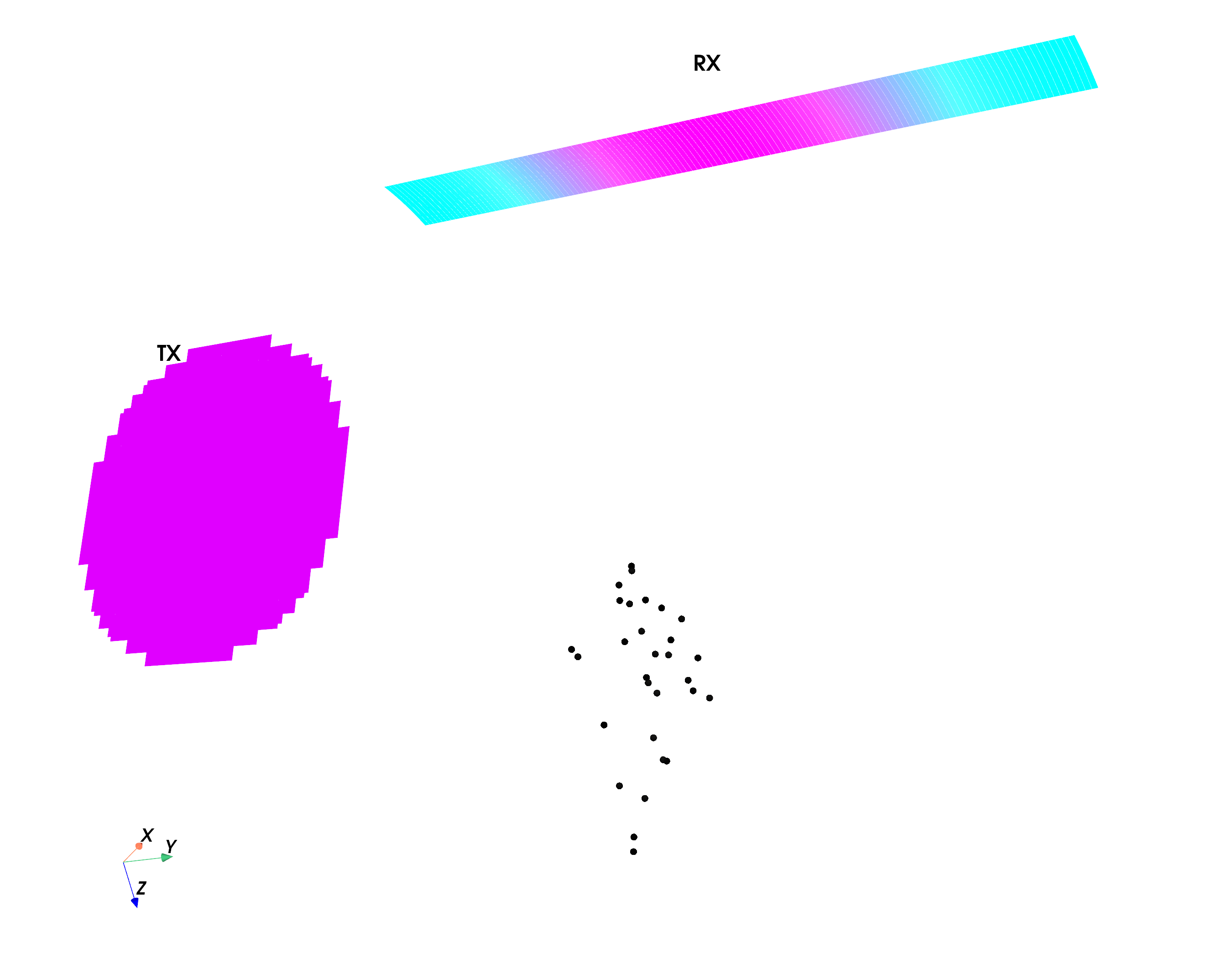
sim.show(scatterer_positions_mm, amplitudes) renders TX/RX meshes and the scatterer cloud in 3-D — run it before a long simulation.

Examples¶

Figure	Study
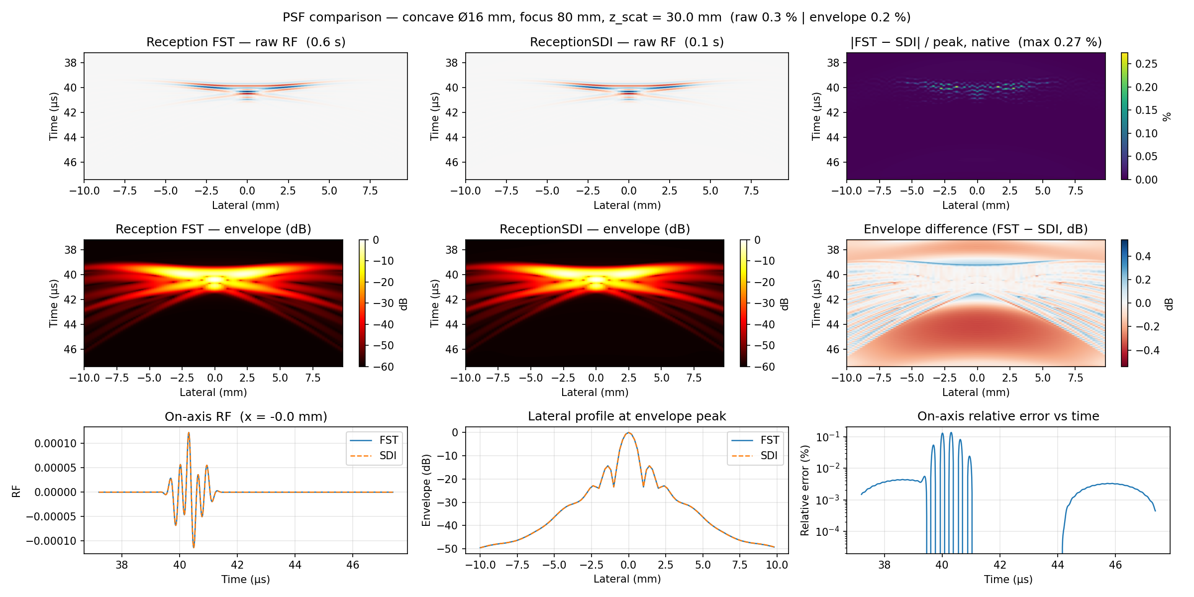	PSF vs Field II
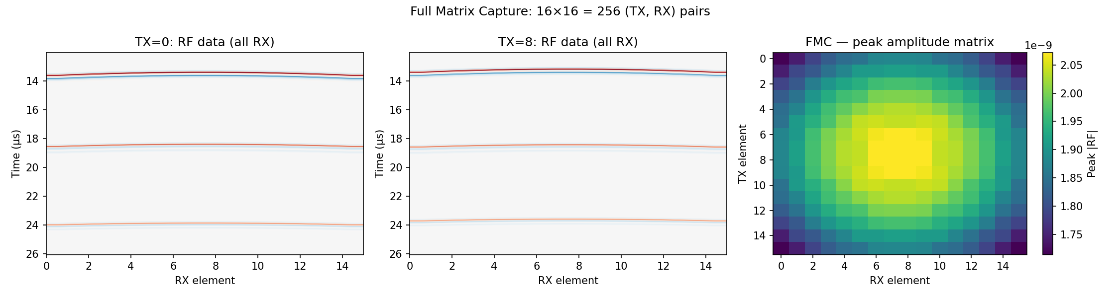	Full Matrix Capture
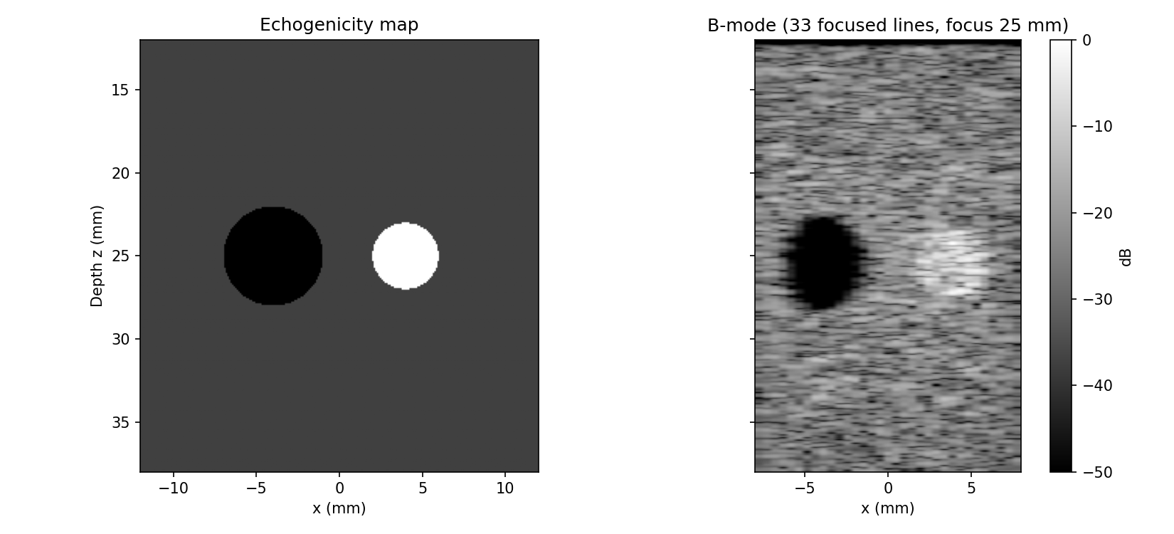	Speckle phantom

Beamforming note¶

coords["t0"] is the beamforming time reference, not the instant of the first RF sample: it is set so a scatterer's echo peaks at its geometric round-trip time (|p − r_tx| + |p − r_rx|)/c. Any beamformer — das_volume, das_rca_volume, or your own — therefore reads the sample at (t_tx + t_rx − t0)·fs with no further correction.

This is the same contract USTB puts in initial_time and MUST's dasmtx assumes, so RF exported with save_rf_hdf5 drops into those workflows unchanged. Getting there costs one shift: the band-limited two-way pulse peaks about half its length after the geometric arrival, and that lag is subtracted from t0 at simulation time. It stays in coords["pulse_center_lag_s"] as provenance — already applied, so adding it again biases the image deep by c·lag/2 (≈0.5 mm for a 2-cycle 5 MHz pulse model).

t_offset_s on the DAS beamformers defaults to 0.0; use it only for RF from elsewhere whose time axis is not referenced this way (raw Field II calc_scat output still carries the lag) or to inject a system delay.

Full signatures: API → Reception · API → Beamforming.