Getting Started
This guide walks you through installing eSDIva and running your first simulation.
Installation
Prerequisites
- Python >= 3.11
- uv (recommended package manager)
Install from PyPI
[all] pulls every optional feature; see Installation for the
slimmer variants.
Install from GitHub
Verify installation
Your first simulation
1. Create a transducer
eSDIva models transducers as collections of rectangular patches. Start with a simple linear array:
from esdiva.transducers import LinearArrayTransducer

tx = LinearArrayTransducer(
    n_elements=64,
    element_width_mm=0.25,
    element_height_mm=12.0,
    kerf_mm=0.05,
    no_sub_x=2,
    no_sub_y=4,
    frequency_Hz=5e6,
)
2. Configure focusing
Set electronic delays and apodization to focus the beam:
3. Define the field grid
Specify the spatial region where pressure will be computed (all distances in mm):
field_points = {
    "x_extent": [-5, 5],
    "y_extent": [-0.5, 0.5],
    "z_extent": [5, 55],
    "dx": 0.1,
    "dy": 1.0,
    "dz": 0.2,
}
4. Run the simulation
from esdiva.emission import Emission

sim = Emission(tx, monochromatic=True)   # continuous-wave amplitude at fc
p, coords = sim(field_points, method="auto")
5. Visualize results
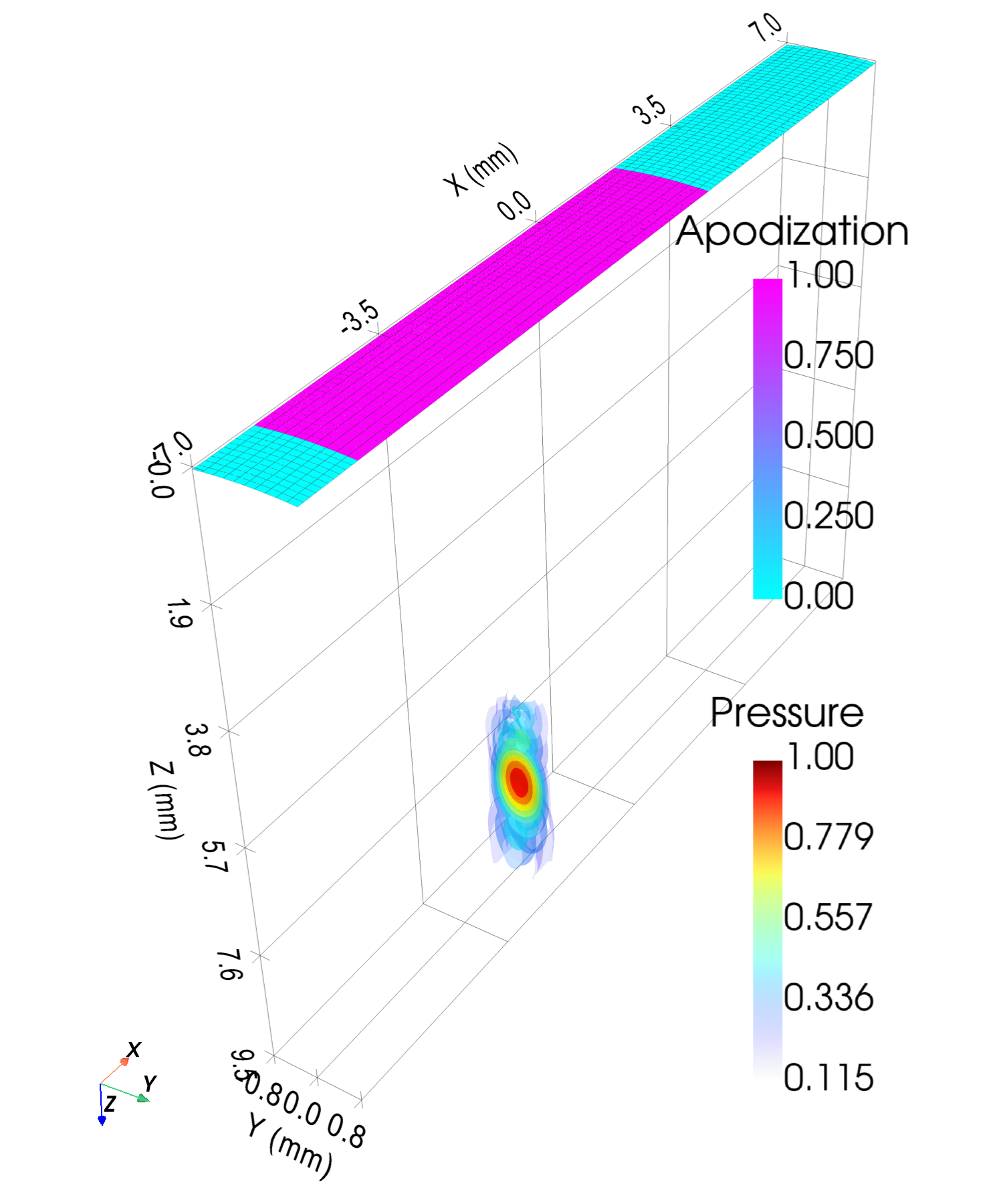
from esdiva.plotting import plot2D_pressure_slices

plot2D_pressure_slices(p, coords=coords, db_scale=True, vmin=-40)
Key concepts
-
Patch-based discretization: every transducer surface is approximated by small flat rectangular patches. The
no_sub_xandno_sub_yparameters control how many patches per element -- more patches means higher accuracy but slower computation. -
Unit convention: user-facing APIs use millimeters (
_mmsuffix); internal computations use SI units (metres, seconds). -
Coordinate system: X = lateral, Y = elevation, Z = axial (depth).
Next steps
- Transducer types -- learn about all available geometries
- Emission -- monochromatic, transient, and attenuated fields
- Reception (RF) -- pulse-echo RF for PSF and phantom studies
- Visualization -- 2D and 3D plotting options