Example 9: B-mode PSF Image via Focused Scan Lines
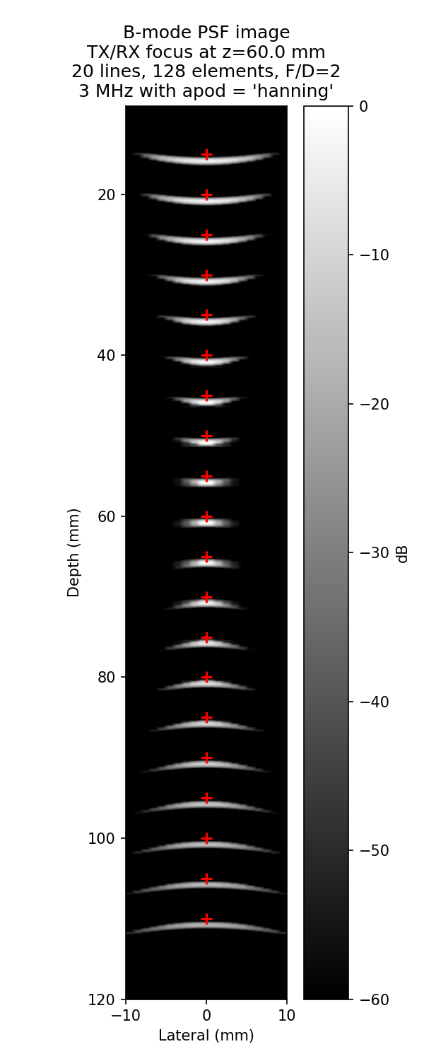
The classic Field II PSF phantom: 20 on-axis point scatterers imaged line by
line with a fixed-focus 128-element array. Each lateral position is one
scan_focusline call — TX focusing, RX beamforming, and envelope detection
happen inside the kernel, exactly like Field II's calc_scat loop.
What you will learn
scan_focusline(focus_mm, scatterers, amps, FoverD, apodization_type)— one focused, apodized, RX-beamformed B-mode line per call- Mapping each line's
coords["t0"]time axis to display depth - Global log compression into a 60 dB B-mode image
Output
Run it
Key code
from esdiva.reception import Reception

sim = Reception(tx, rx, c=1540, fs=100e6, excitation=pulse)

env_lines = []
for x in x_lines_mm:
    env, coords = sim.scan_focusline(
        [x, 0.0, 60.0], scatterer_pos, scatterer_amp,
        FoverD=2.0, apodization_type="hanning",
    )
    depth_mm = (coords["t0"] + np.arange(len(env)) * coords["dt"]) * 1540 / 2 * 1e3
    env_lines.append(np.interp(common_depth_mm, depth_mm, env, left=0, right=0))

bmode = 20 * np.log10(np.maximum(np.stack(env_lines, 1) / peak, 1e-3))