Example 22: Ultrafast Compound Doppler
A controlled replication of ultrafast compound Doppler imaging — Bercoff, Montaldo, Loupas, Savery, Mézière, Fink & Tanter, IEEE Trans. Ultrason. Ferroelectr. Freq. Control 58(1):134–147, 2011 — run on a phantom whose true velocity we set ourselves, which the original experiment could not have.
The claim: a colour-flow image built from a handful of tilted plane waves, coherently summed, gives the same Doppler performance as conventional line-by-line focused Doppler for 8× fewer emissions here. One phantom, one probe, one pulse, one Doppler PRF, one estimator, one noise level — only the transmit differs.
| Sequence | Transmit | Emissions | Slow-time samples |
|---|---|---|---|
| Conventional focused | 72 focused lines, one packet each | 576 | 8 |
| Compounded ultrafast | 9 tilted plane waves per frame | 72 | 8 |
| …long ensemble | 9 tilted plane waves per frame | 288 | 32 |
What you will learn
- Moving scatterers —
scatterer_positions_mmas(N_emissions, N_scat, 3), one cloud per emission; eSDIva has no slow-time clock, so you write the trajectory - The design rule
N_angles = PRF_max/PRF_doppler, and how the depth limitPRF_max = c/(2·z_max)makes every extra angle cost velocity range - Why compounding happens within a frame and never across frames — summing across frames averages away the phase that carries the flow
- Designing the elevation aperture — the axis the image cannot show, and the one that decides whether a velocity number is trustworthy
- Sizing a phantom by scatterers per resolution cell, not by total count
Output
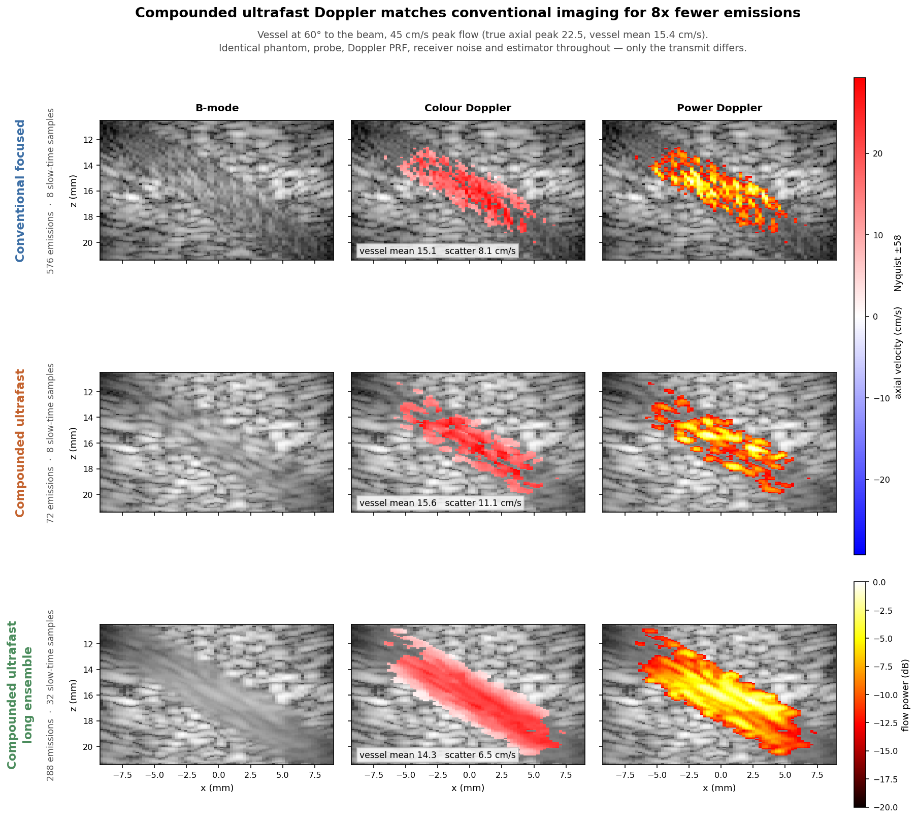
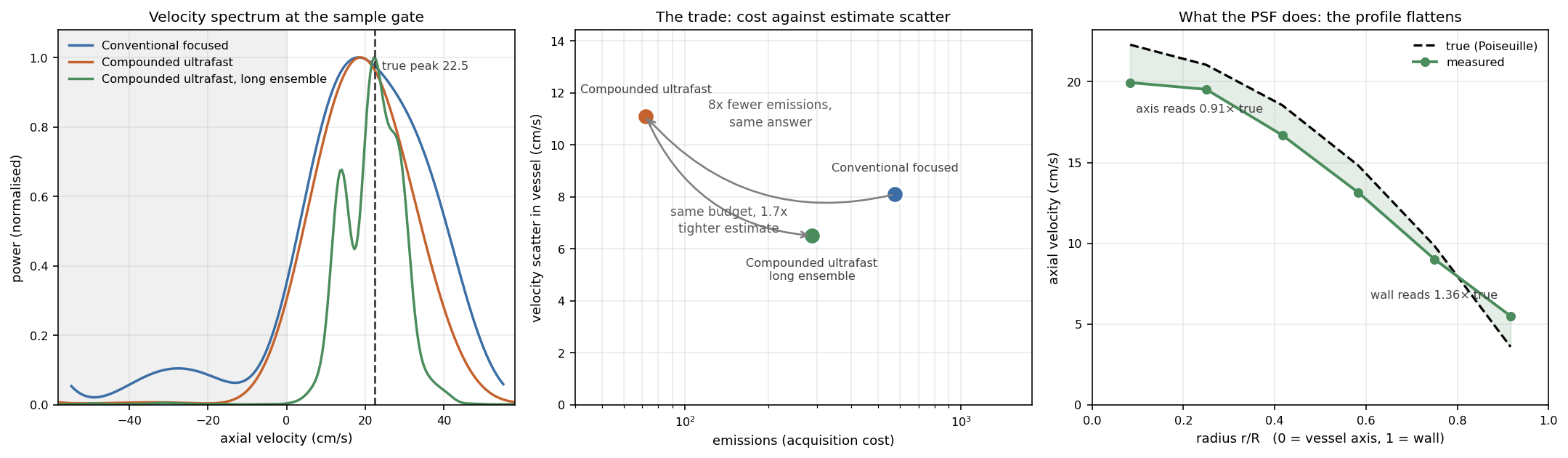
Each row is one sequence: the B-mode it reconstructed, its colour Doppler map on a shared velocity scale, and its power Doppler.
The flow, frame by frame
Blood is barely visible on the B-mode — that is the point, and why Doppler exists. The colour overlay comes from the same frames, and the velocity profile across the tube is read from the map, not from the phantom's definition.
What the transmit costs
Both panels are real beamformed output. The conventional scan builds its image one focused line at a time; the ultrafast one shows each tilted plane wave and their coherent sum, at nine emissions per frame against 72 lines.
Rebuild both with uv run examples/example22_flow_doppler/make_videos.py once
step 2's RF is on disk.
Run it
uv run examples/example22_flow_doppler/step1_define_flow_phantom.py   # preview
uv run examples/example22_flow_doppler/step2_acquire_RF.py            # the long one
uv run examples/example22_flow_doppler/step3_doppler_processing.py
uv run examples/example22_flow_doppler/step4_visualize.py
Step 3 asserts both of the paper's claims, so the example fails loudly if the simulator, the beamformer or the estimator regresses.
Estimate the runtime on your own machine first
Step 2 calls esdiva.utilities.estimate_sequence_runtime, which times short
probes on the real phantom and projects. Cost per emission is a property of
the hardware and varies by more than an order of magnitude between a laptop
and a compute node. Every run is checkpointed, so a killed job resumes.
Key code
# Events are just transmit delays. Copy them - probe.delays is live state.
frame = []
for angle in ANGLES_DEG:
    probe.compute_delays(angle_steering_deg=float(angle))
    frame.append({"delays": np.asarray(probe.delays, np.float32).copy(),
                  "apodization": np.ones(N_ELEMENTS, np.float32),
                  "angles_deg": float(angle)})
events = frame * ensemble          # the SAME angles every frame

# One scatterer cloud per emission - this is what makes flow possible.
positions = np.stack([np.vstack([tissue, blood_at(m)])
                      for m in range(n_emissions)])       # (N_em, N_scat, 3)
rf, coords = sim.sequence_rf(positions, amplitudes, events, out_path="out/RF_B")

# Compound WITHIN a frame; each frame is one slow-time sample.
for k in range(ensemble):
    sl = slice(k * N_ANGLES, (k + 1) * N_ANGLES)
    vol, gc = das_volume(rf[sl], {...}, frame_events, probe, GRID_MM, c=C)

f_echo = echo_center_frequency(beamformed, 1 / fs_depth, band=(0.3 * FC, 1.7 * FC))
iq = rf2iq(beamformed, fs_depth, f_echo)
v_map, power = iq2doppler(wfilt(iq), PRF_DOPPLER, f_echo, c=C)
The Doppler chain (rf2iq, wfilt, iq2doppler) lives in the example, not the
package — eSDIva simulates the RF and beamforms it; turning an ensemble into a
velocity is signal processing. See
Flow Simulation.
Two things worth sizing before you run
The folder's own README.md carries the measurements and the error budget.
- Size the phantom by scatterers per resolution cell, and the cell against the vessel. Too few per cell gives a moth-eaten flow map; a cell too large beside the lumen flattens the profile. Elevation is the axis that bites, since a linear array does not focus there electronically — an elevation lens is the fix.
- Add receiver noise before any sensitivity claim. eSDIva's RF is noiseless by
design, so a longer ensemble has nothing to average down. Use
esdiva.utilities.add_noisewith one sharedreferenceacross the sequences being compared — noise belongs to the receiver, not the transmit scheme.