PSF Simulation
The point-spread function is the echo a single point target sends back — the impulse response of the whole imaging chain, transmit aperture through receive aperture. Everything an image does to a scatterer, it does through this: spatial resolution, sidelobe level, depth of field, and the clutter that fills an anechoic target are all readable from the PSF before a single phantom is drawn.
per_scatterer=True is the whole difference. Without it the echoes of all
targets are summed into one (Erx, Nt) record, as a real acquisition would;
with it each target keeps its own (Erx, Nt) page, so target p can be
beamformed, enveloped and measured in isolation.
Choosing the points
Two ways in, and they mean different things:
# 1. Explicit targets: a few wires at known depths.
pts = np.array([[0, 0, 20], [0, 0, 30], [0, 0, 40]], dtype=float)
psf, coords = sim.pulse_echo_rf(pts, per_scatterer=True)

# 2. A grid dict — the same x_extent/dx form emission uses — giving a regular
#    lattice of unit-amplitude targets, one PSF page each.
grid = {"x_extent": [-5, 5], "y_extent": [0, 0], "z_extent": [15, 45],
        "dx": 1.0, "dy": 1.0, "dz": 5.0}
psf, coords = sim.pulse_echo_rf(grid, per_scatterer=True)
A lattice is not a phantom
A regular grid of scatterers returns coherent echoes: the targets are
periodic, so their contributions add in phase along certain directions and
produce interference patterns that look like artefacts but are not. That is
exactly what you want for mapping a PSF over a field of view, and exactly
what you must not use for speckle. For tissue, draw random positions with
make_phantom.
Set the impulse responses first
A PSF measured without tx.impulse_response and rx.impulse_response is a
different PSF. A physical probe band-passes twice — drive ⊛ TX piezo ⊛ RX piezo —
and skipping the two responses simulates ideally broadband elements, which lets
the low-frequency tails of the aperture diffraction responses dominate the
received spectrum. Measured consequences: the received centroid drops (3.0 →
1.86 MHz in one study), the lateral PSF widens ~60 %, and the near-in sidelobe
skirt rises from −22 to −10 dB, where it becomes the dominant clutter in a
volume.
t = np.arange(0, 2 / fc, 1 / fs)                 # 2-cycle burst at fc
ir = np.sin(2 * np.pi * fc * t) * np.hanning(len(t))
tx.impulse_response = ir
rx.impulse_response = ir
Symptom to recognise: point targets 50–100 % wider than λz/D while every
arrival time is geometrically exact. That is a spectrum problem, not a
beamformer problem.
Reading the result
from esdiva.beamforming import das_volume, envelope_db

vol, gc = das_volume(psf[p][None], coords, [event], rx, grid_mm, c=1540)
img = envelope_db(vol)
Measure lateral and axial FWHM at −6 dB, and the sidelobe level over a window
wide enough to include the first few lobes. Scale every ROI and exclusion margin
in PSF units (λz/D at the target's depth), never in millimetres — a
fixed-mm ROI silently changes meaning the moment the probe or the depth changes,
which is the usual reason metrics "collapse" on a new probe.
One focused line, RX summed in the kernel
scan_focusline is the conventional-scanner shortcut: it fires one focused
transmit and returns a single beamformed line, summing the receive channels
inside the kernel rather than handing you channel data.
env, coords = sim.scan_focusline([0, 0, 30], pts, amp,
                                 FoverD=2.0, apodization_type="hanning")  # (Nt,)
Cheaper than a full pulse_echo_rf when the line is all you want, and it is the
direct counterpart of Field II's calc_scat.
Worked examples
| Figure | Study |
|---|---|
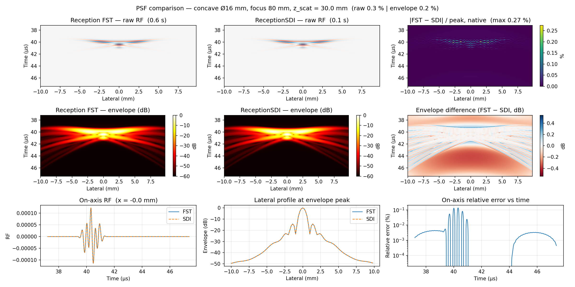 |
PSF vs Field II — correlation ~1.0 against the reference |
Full signature: API → Reception.