Example 4: Linear Array — Diverging Wave (Transient)
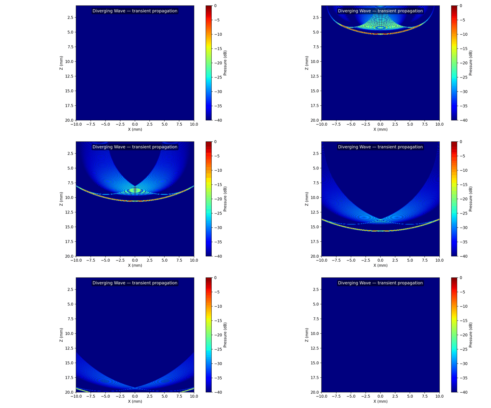
Pulsed emission of a diverging wave: a virtual source behind the array produces the wide unfocused beam used in ultrafast imaging. The full spatio-temporal pressure field is computed and animated.
What you will learn
- Diverging-wave delays from a virtual focus at
z < 0 - Defining a Hanning-windowed excitation pulse
- Transient
Emissioncalls → pressure shape(Nt, Nx, Ny, Nz) - Reconstructing the time axis from
coords["t0"]/coords["dt"] - Animating the wavefront with
plot2D_pressure_slices
Output
Run it
Key code
import numpy as np
import esdiva.transducers as transducers
from esdiva.emission import Emission
from esdiva.plotting import plot2D_pressure_slices

tx = transducers.Domino()
tx.compute_delays(focus_mm=[0, 0, -10])  # virtual focus behind the array

# 2-cycle Hanning-windowed excitation at the probe centre frequency
t_pulse = np.arange(0, 2 / tx.fc, 1 / 200e6)
excitation = np.sin(2 * np.pi * tx.fc * t_pulse) * np.hanning(len(t_pulse))

sim = Emission(tx, fs=200e6, excitation=excitation)
p, coords = sim(plane_config)          # (Nt, Nx, Ny, Nz)

t = coords["t0"] + np.arange(p.shape[0]) * coords["dt"]
plot2D_pressure_slices(p, coords=coords, time_array=t, db_scale=True, vmin=-40)