Mono-element Transducers¶

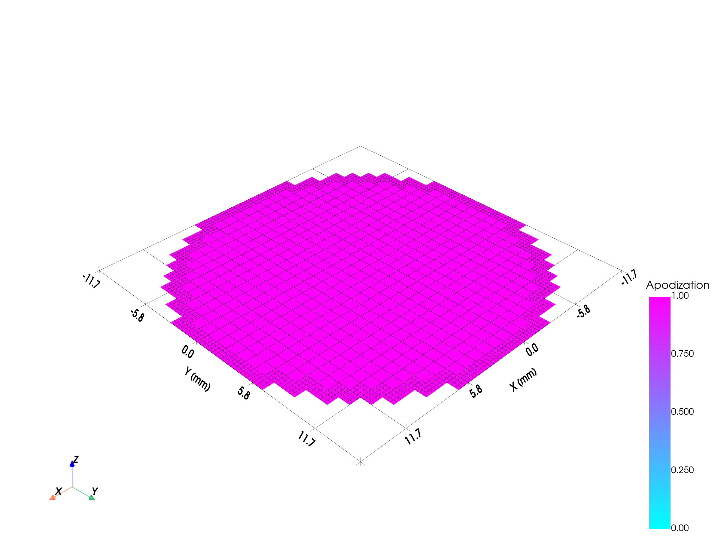
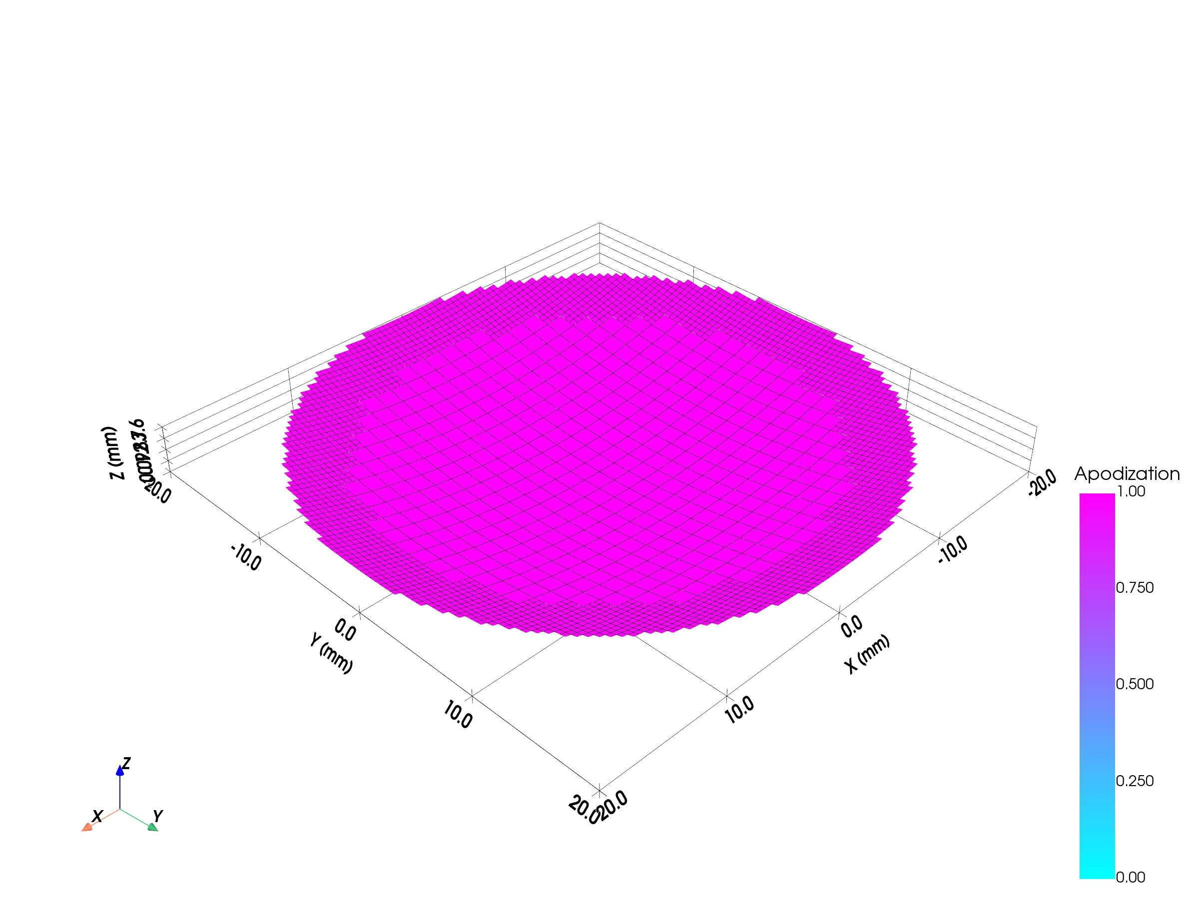
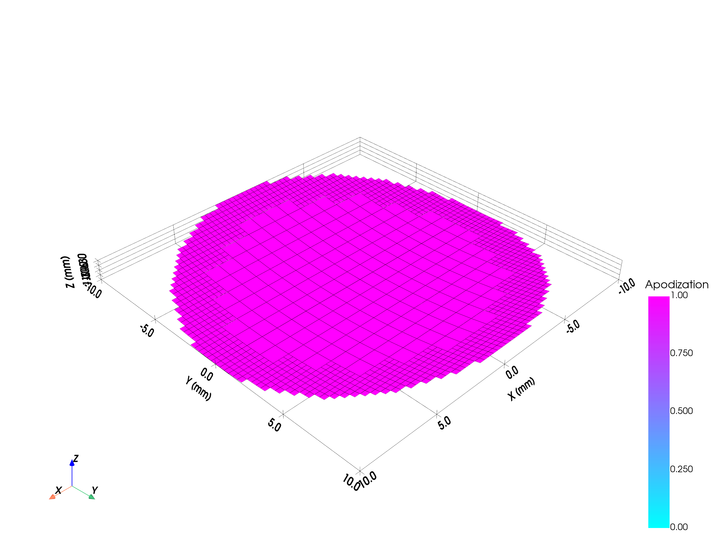
Single-element circular transducers. Focusing comes from the physical curvature of the surface, not electronic delays. See the Transducers API for full parameters and Example 2 — Mono-element Fields.

The radiated pressure fields for these transducers live in the Emission guide.

At a glance¶

All mono-element transducers have n_elements = 1. Electronic delays have no effect — focusing is achieved through the physical curvature of the surface.

Z-convention¶

For all curved circular transducers the rim is at z = 0. The focus_mm parameter sets the axial depth from the rim to the geometric focus:

tx = ConcaveCircularTransducer(
    diameter_mm=64.0,
    focus_mm=63.0,   # radius of curvature = focal length (datasheet Rfocus)
    frequency_Hz=0.5e6,
    no_sub_diameter=30,
)

For the spherical caps focus_mm is the radius of curvature (= focal length, the datasheet Rfocus): with the apex at z = 0 the geometric focus lands at z = focus_mm, so here radius and focal depth coincide. focus_mm = D/2 gives a hemisphere. (The linear-array elevation_focus_mm uses the same radius convention but a rim datum, so there they don't coincide — see Multi-element § Elevation lens.)

Arbitrary radial profiles¶

ConcaveCircularTransducer and ConvexCircularTransducer are the two spherical cases of a more general element: any axisymmetric cap z(r). When the surface is not a sphere — an aspheric lens, a refractive doublet, a measured profile — describe it directly with RadialProfileTransducer, giving the radial sag as a callable z(r) in mm:

from esdiva.transducers import RadialProfileTransducer

# A shallow convex (diverging) cap: z dips as r grows.
tx = RadialProfileTransducer(
    diameter_mm=0.6,
    surface_sag_mm=lambda r: -0.05 * r**2,   # z(r) in mm, any axisymmetric profile
    frequency_Hz=15e6,
    no_sub_diameter=40,
)

It tiles the surface into rectangular patches with the same ring-based subdivide_radial the spherical caps use (see Geometry Functions), so flat piston, bowl, dome and aspheric profiles share one engine — the circular classes are convenience wrappers around a fixed spherical z(r). The highest point of the profile is pinned to z = 0; a pure z-shift leaves the far-field directivity unchanged.

For a non-spherical cap there is no single centre of curvature, so a beamformer cannot assume the aperture plane is the acoustic origin. tx.virtual_source_m returns the point the cap effectively radiates from — the paraxial centre of curvature, computed from geometry alone (no field simulation) — which is where delay-and-sum should reference the element. Fitting such a profile to a target directivity, and using its virtual_source_m for imaging, is Example 23 and Example 24.