Flow Simulation¶

Doppler does not measure a frequency shift inside one echo. It measures the phase an echo gains between emissions, because the blood moved v/PRF in between: a scatterer receding by Δz lengthens the round trip by 2Δz, turning the echo phase by 4π·f·Δz/c. Every Doppler estimator there is stacks those increments over an ensemble.

sequence_rf reproduces exactly that by taking one scatterer cloud per emission — (N_events, N_scat, 3) instead of (N_scat, 3).

t = np.arange(n_events) / prf                        # slow-time, s
pos = pos0[None] + v_mm_s[None] * t[:, None, None]   # (N_events, N_scat, 3)
rf, coords = sim.sequence_rf(pos, amp, events, out_path="rf_store")

ndim disambiguates, so a static call is unchanged. eSDIva has no slow-time clock of its own, and that is deliberate: because the trajectory is yours to write, a pulsatile, cardiac, recirculating or decorrelating flow is no harder than a constant one — the same call, a different array.

amplitudes may vary per event too, as (N_events, N_scat). The scatterer count is fixed across the sequence, so setting an amplitude to zero is how a scatterer that has left the region of interest is retired — and how a contrast bubble is destroyed. Checkpointing, resume and the config fingerprint all work unchanged; the fingerprint hashes the positions by value, so two different flows cannot be mixed into one store.

What the model resolves

Scatterers are frozen during each emission. Motion is resolved at the event rate, so the RF carries the phase shift between emissions — exactly what a Doppler estimator reads — and not an intra-pulse frequency shift. Velocities of clinical interest move a small fraction of a wavelength during one pulse, which is why this is the standard flow model and the same boundary Field II works within.

The two limits to design against¶

Aliasing. The unambiguous axial velocity is v_nyquist = c·PRF/(4·fc). Beyond it the inter-emission phase leaves ±π, and the estimate folds and reverses sign.
Beam-to-flow angle. Only the axial component is visible: flow returns v·cos θ, and flow perpendicular to the beam returns nothing at all. A Doppler image of a perpendicular vessel is legitimately blank, so tilt the vessel and recover v·cos θ as your ground truth.

For a compounded sequence the two limits meet the depth limit in one design rule:

N_angles = PRF_max / PRF_doppler          PRF_max = c / (2·z_max)

You cannot fire again until the last echo is back, so every extra angle is paid for out of the velocity range. Compounding is never free.

What eSDIva does and does not ship¶

The simulator produces the RF; the beamformers turn it into frames. Turning an ensemble of frames into a velocity is signal processing, not acoustics, so eSDIva ships no Doppler estimator and no clutter filter — the flow & Doppler example writes both in a few lines of numpy each, kept in the open so every assumption behind a velocity number is visible:

beamformed RF  ->  rf2iq  ->  wfilt  ->  iq2doppler  ->  velocity

The names and the signatures are the conventional ones, so code written against another ultrasound toolbox transfers with its argument order intact: rf2iq(RF, Fs, Fc) demodulates to I/Q and estimates Fc itself when it is omitted (rf2iq(RF, Fs)), returning it alongside the I/Q on request; wfilt removes the clutter; iq2doppler returns velocity and power.

iq, fc = rf2iq(beamformed, fs_depth, return_fc=True)   # Fc estimated
v, power = iq2doppler(wfilt(iq), prf, fc)

Give Fc explicitly for undersampled RF

Under bandpass sampling the carrier is aliased and cannot be recovered from the spectrum, so the estimate would be wrong. Pass the known Fc.

What is inside rf2iq

Four different things get loosely called "IQ", and a Doppler chain that confuses them fails in ways that look like physics:

Object	Real/complex	Centred at	Phase
RF	real	`fc`	in the carrier
Analytic signal — `scipy.signal.hilbert(rf)`	complex	`fc`	kept
Baseband IQ — analytic × `exp(-j2π·fc·t)`	complex	0	kept
Envelope — `abs(analytic)`	real	0	discarded

Doppler runs on baseband IQ (or equivalently on the analytic signal). It can never run on the envelope: the phase is the signal. scipy.signal.hilbert is misleadingly named — it returns the analytic signal, not the Hilbert transform.

Worked example¶

One acquisition, three readings of it: the B-mode where the blood is all but invisible, the colour Doppler map built from the same frames, and the velocity profile across the vessel.

Figure	Study
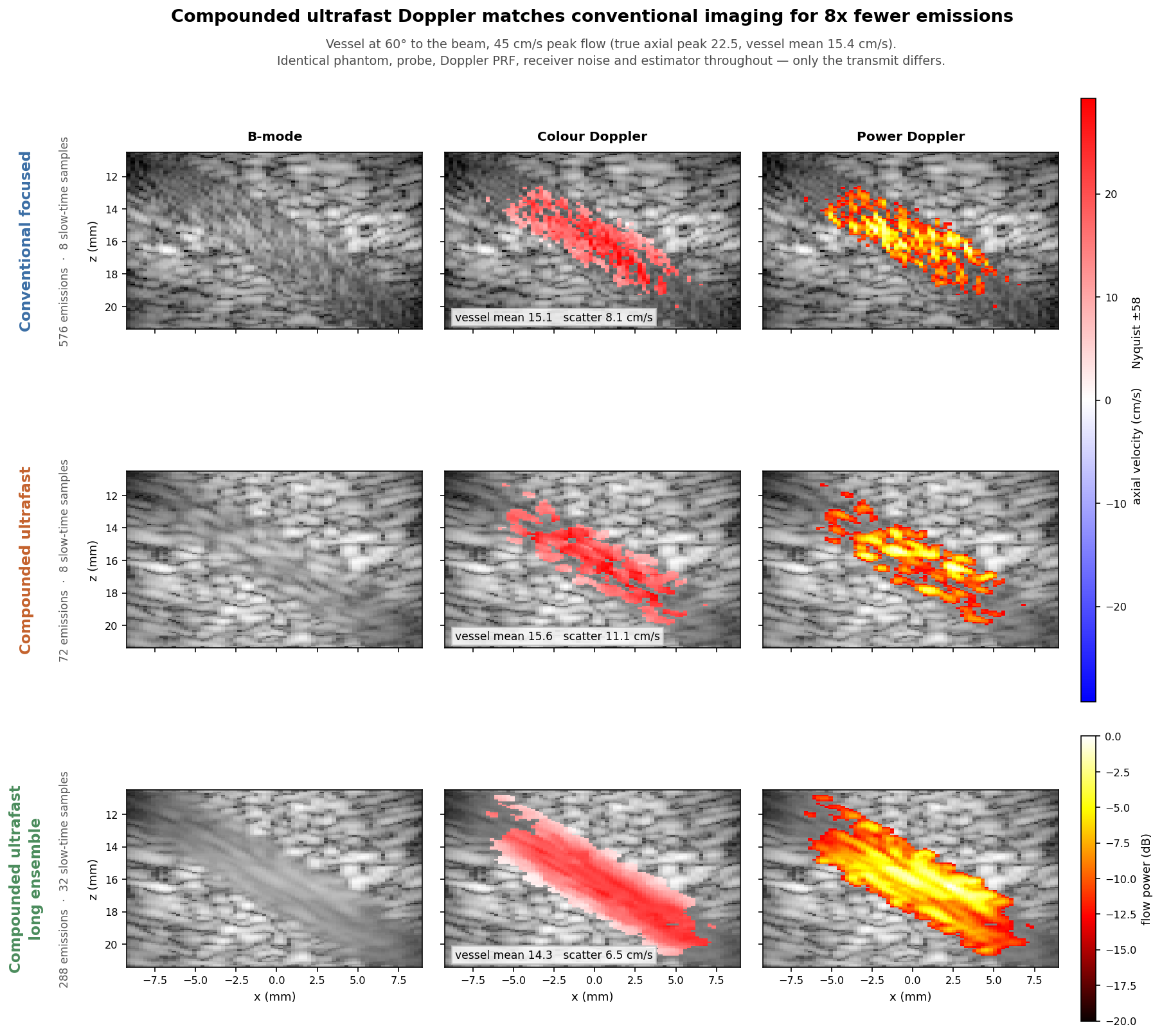	Ultrafast compound Doppler — a replication of Bercoff et al. (2011) against a known velocity field

Full signature: API → Reception.