Emission
Emission computes the pressure field radiated by a transducer. One callable
covers four modes, selected by constructor flags; __call__ always returns
(pressure, coords).
from esdiva.emission import Emission

sim = Emission(tx, monochromatic=True)          # |P(r, fc)| → (Nx, Ny, Nz)
sim = Emission(tx)                              # pulsed transient (raw SIR) → (Nt, …)
sim = Emission(tx, fs=200e6, excitation=exc)     # global excitation (L,)
sim = Emission(tx, fs=200e6, excitation=exc_LE)  # per-element excitation (L, E)

p, coords = sim(field_points)                    # method: None = fastest for the mode
Physics: P(r, ω) = ρ₀ · jω·V(ω) · H(r, ω) — the velocity pulse v (excitation ⊛
impulse response) times the aperture's spatial impulse response H. Transfer functions
(attenuation, a user transfer_function, per-element drives) multiply in the same
frequency domain. Transient pressure is signed (compression > 0, rarefaction < 0)
and in pascals for rho in kg/m³ and a velocity in m/s, independent of fs.
Algorithmic flow
flowchart LR
    T[Transducer<br/>delays · apodization · baffle] --> E[Emission<br/>c · rho · fs · alpha0]
    E --> S{SIR source}
    S -->|spectral| H["closed-form H(ω)"]
    S -->|temporal / fst / auto| h["sampled h(t) → FFT"]
    H --> F["× jω·V(ω) × TF × H_att"]
    h --> F
    F -->|monochromatic| M["|P| at exactly fc"]
    F -->|transient| I["irfft → signed p(t)"]
Modes at a glance
| Constructor | Output | coords |
Page |
|---|---|---|---|
monochromatic=True |
(Nx, Ny, Nz), ρ·ωc·\|H\| per 1 m/s |
x, y, z |
Monochromatic |
default (excitation=None) |
(Nt, Nx, Ny, Nz), ρ·h(t) |
+ t0, dt |
Transient Impulse |
excitation=(L,) or (L, E) |
(Nt, Nx, Ny, Nz), signed Pa |
+ t0, dt |
Transient + Excitation |
alpha0=… |
as above | as above | Attenuation |
Raw (N, 3) input drops the spatial axes: (N_points,) / (Nt, N_points).
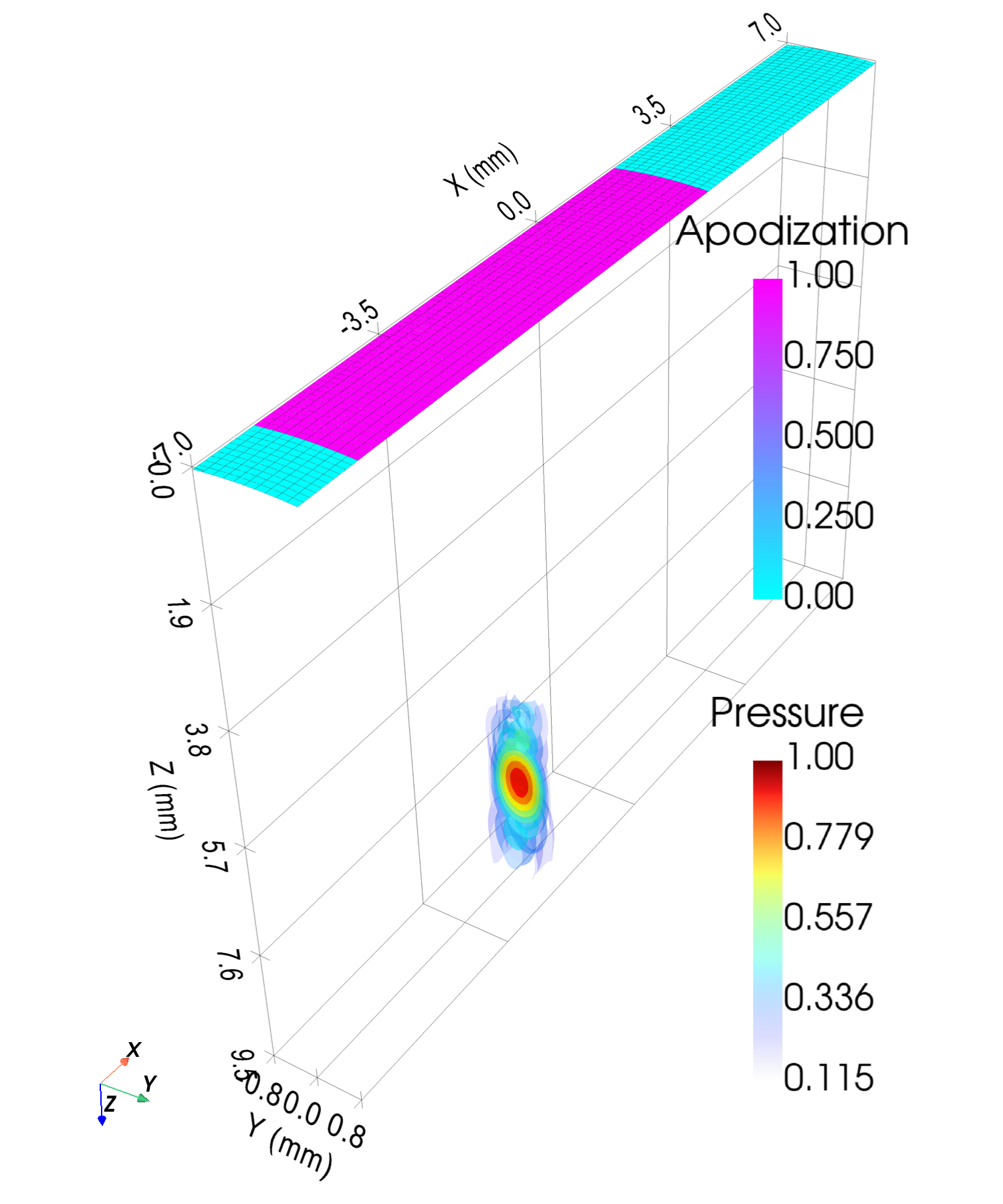
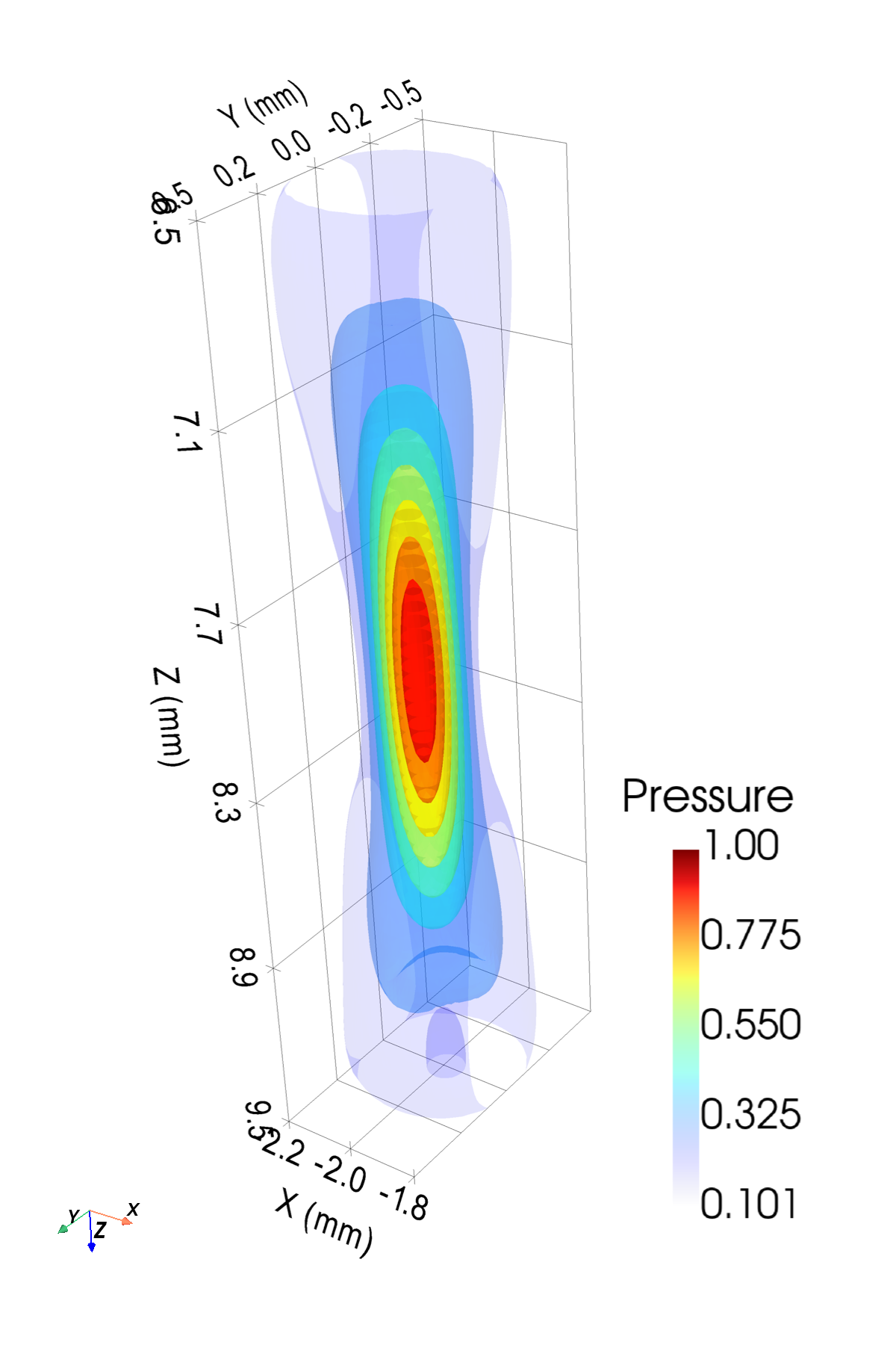
Monochromatic field
Steady-state amplitude at exactly the centre frequency — ideal for beam patterns and focal-spot characterisation.
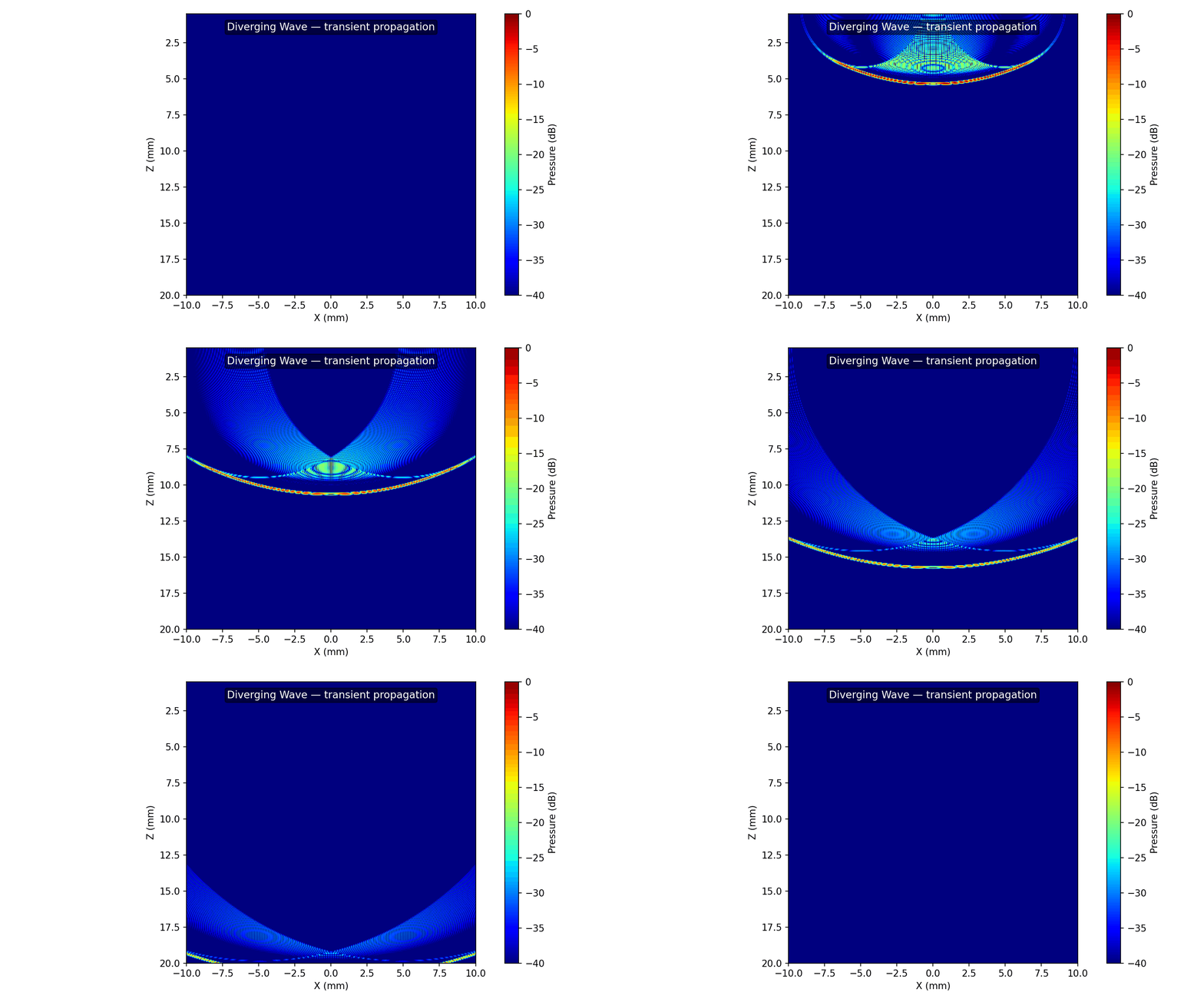
Transient field
Convolve the SIR with an excitation pulse for the full time-domain wavefront — diverging waves, steered plane waves, propagation snapshots.
SIR source: spectral or temporal
Both evaluate the same far-field trapezoidal SIR and agree to about 1 %:
"spectral"— the closed-form spectrumH(ω)(per patch: area × two sincs × a delay phasor), exact, evaluated only on the pulse's frequencies."temporal"(="sdi"),"fst","auto"— the sampledh(t), then an FFT.
The default method=None picks the faster: spectral for monochromatic fields and for
per-element drives or attenuation, temporal for every other transient field.
Key parameters
| Parameter | Role |
|---|---|
monochromatic |
Amplitude at fc vs transient waveform |
excitation |
None (raw SIR), (L,) global, or (L, E) per-element |
fs |
Time sampling for transient output |
alpha0, freq_power |
Power-law attenuation (see Attenuation) |
fast_attenuation |
Attenuation path from the transducer centre (True) or each element |
transfer_function |
Extra frequency response TF(f) (applied at fc in monochromatic mode) |
method |
None (fastest), "spectral", "temporal", "fst", "auto" |
tx.baffle |
"rigid" (default) or "soft" (cosθ obliquity per patch) |
Full signature and every parameter: API → Emission.