Phantom Simulation¶

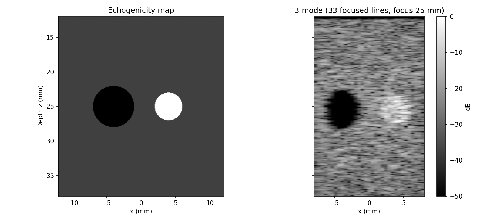
A phantom is a cloud of random scatterers whose amplitudes follow the echogenicity you want to image. Randomness is the point: it is the interference of many sub-resolution scatterers that produces speckle, and speckle is what a B-mode image is mostly made of. A regular lattice returns coherent echoes instead, which look like an image but obey none of the statistics that contrast and texture measurements assume.

from esdiva.utilities import make_phantom

pos, amp = make_phantom(extents_mm, n=20000, echogenicity_map=my_map)
rf, coords = sim.pulse_echo_rf(pos, amp)

make_phantom draws uniform random positions inside extents_mm and gives each one an N(0, 1) amplitude scaled by echogenicity_map(r) — zero inside an anechoic lesion, larger inside a bright one. The Gaussian draw is what makes the envelope Rayleigh-distributed, as it is in tissue.

Use sequence_rf, even for one event¶

sequence_rf is the recommended entry point for any phantom study, static or moving. The same RF is reachable by calling pulse_echo_rf once per transmit and stacking the results — the physics is identical — but the loop gives you none of the operational guarantees a multi-hour acquisition needs:

• Checkpointing. With out_path=, each event lands on disk the moment it finishes, so a crash or a killed job costs at most the event in flight, and re-running resumes at the first missing one. A hand-rolled loop that dies in hour six has produced nothing.
• A config fingerprint. The store records probe, medium, excitation, scatterers and events; re-running with any of them changed raises with a diff instead of silently mixing incompatible data into one dataset.
• checkpoint_chunks= bounds the loss within one event, with zero-amplitude grid sentinels that pin one time grid per event so the partial RFs sum exactly.
• Per-event time origins, collected into coords["t0_per_event"] and consumed directly by the beamformers.

rf, coords = sim.sequence_rf(pos, amp, events, out_path="rf_store",
                             checkpoint_chunks=4)

from esdiva.io import RFDataset

ds = RFDataset("rf_store")
ds.summary()                     # what is done, what is missing
rf, coords = ds.load_all()
ds.to_hdf5("channels.h5")        # UFF-compatible fields for MATLAB / USTB

pulse_echo_rf stays the right call for a single acquisition or a PSF map; it accepts the same out_path= and routes through sequence_rf internally, so it inherits the same guarantees.

Designing the phantom¶

• Speckle density — at least ~5–10 random scatterers per resolution cell (λz/D)² · (pulse length)/2. Below that, the texture and every contrast number you compute from it are artefacts of the particular random draw rather than properties of the imaging system. Cell volume scales as ~λ³, so a 10 MHz probe needs roughly 50× more scatterers than a 3 MHz one for the same box.
• Anechoic targets — radius ≥ ~3 PSF widths, or the lesion fills in from its own blurred edges and the contrast you measure is the blur, not the lesion.
• Wires — coherent within a resolution cell, so their brightness scales with PSF volume rather than with scatterer count. Keep them dim (~+10 dB over speckle), few, and far from any contrast target.
• Preview before burning hours — sim.show(pos, amp) renders the cloud with the apertures, then run one event and check the envelope statistics (Rayleigh gives mean/std ≈ 1.91) before launching the full sequence.

from esdiva.utilities import estimate_sequence_runtime
est = estimate_sequence_runtime(sim, pos, n_emissions=n_angles * n_frames)

Beamforming the result¶

from esdiva.beamforming import das_volume, envelope_db

vol, gc = das_volume(rf, coords, events, rx, grid_mm, c=1540, fnum=1.0)
img = envelope_db(vol)

A few things that decide whether the numbers are honest:

• Rect receive apodization. Elements roughly λ wide already taper the aperture through their own directivity; adding a Hann receive taper on top halves the effective aperture (measured 0.98 vs 0.52 mm FWHM). Prefer a rect taper and a low f-number.
• TGC from speckle-only regions, applied depth-only, never estimated across an anechoic target.
• Report plain DAS. Coherence-factor weighting recovers contrast numbers but destroys speckle texture and passes coherent clutter — quote it as a ceiling, not as the result.
• ~30 dB display window. After TGC, speckle fills about 30 dB; a 40+ dB window makes perfectly normal sidelobes look like artefacts.

Worked examples¶

Figure	Study
	Speckle phantom
	Full Matrix Capture

Full signature: API → Reception · API → Beamforming.